Methods

All three methods share the same interface and return type. Switch methods by passing a different algorithm struct as the first argument to disaggregate.

Comparison

Benchmarks: 20-year span, output_period=Week(1), 8 threads (Julia 1.12). Time = minimum over 2–3 runs. Memory = dominant working-set matrix (n × matrix_width × 8 B).

Method	Pros	Cons	n = 10k	n = 100k	n = 1M
Spline	No kernel required; optional tension suppresses oscillation near sparse gaps	Design matrix O(n × n_knots); can oscillate without tension	12 ms<br>19 MB	103 ms<br>192 MB	807 ms<br>1.9 GB
Sinusoid	Analytical integrals (no quadrature); interpretable parameters (amplitude, phase, trend, anomalies); lowest peak memory	Assumes annual periodicity; poor fit for non-sinusoidal signals	61 ms<br>2 MB	133 ms<br>19 MB	2.4 s<br>192 MB
GP	Arbitrary KernelFunctions.jl kernels; most flexible	O(n·m·q + m³) Cholesky — memory-limited above n ≈ 50 000 at weekly output	2.0 s<br>195 MB	13.3 s<br>1.9 GB	—<br>(>8 GB)

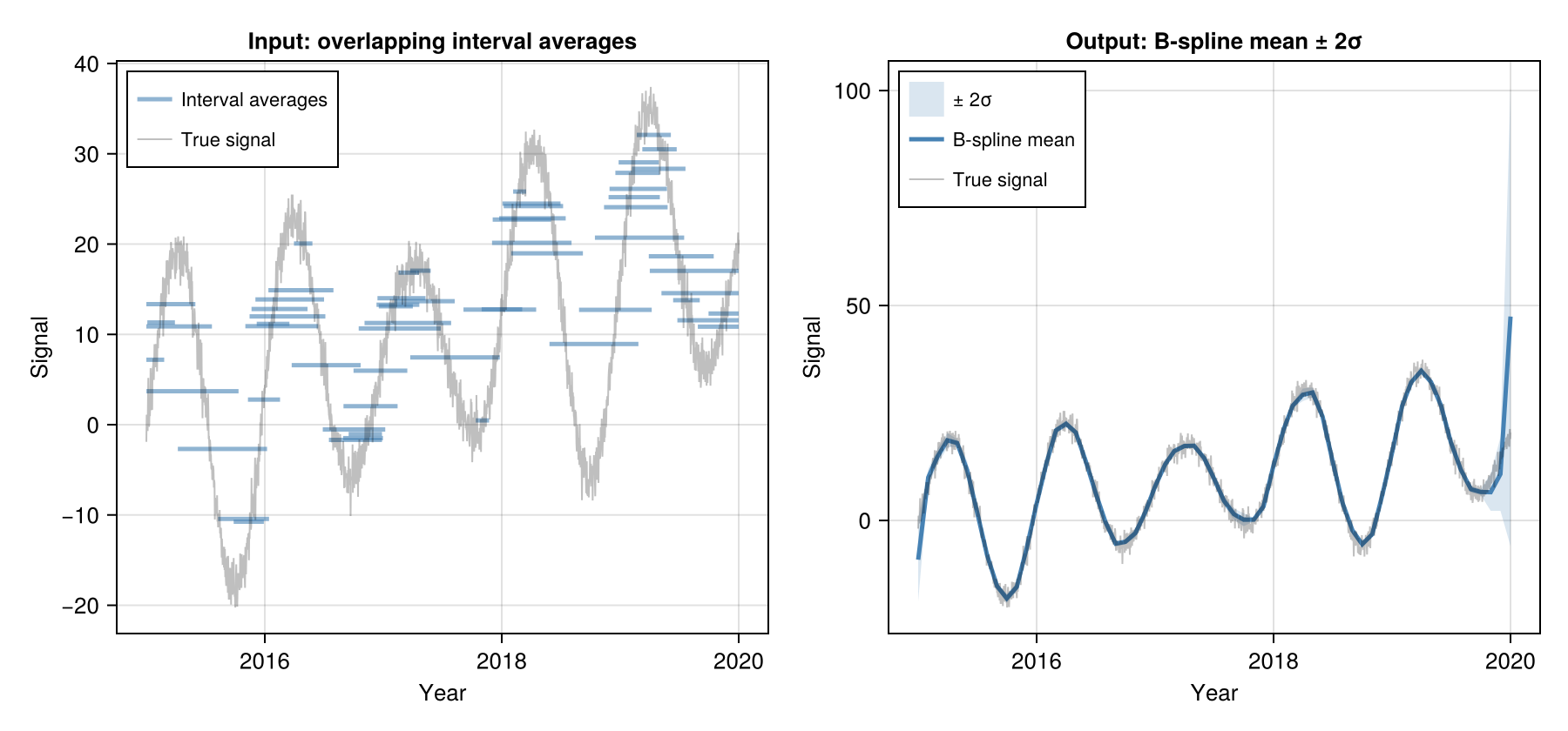
B-spline (Spline)

Fits a smooth curve whose running averages match the observations. A regularisation parameter controls smoothness; an optional tension penalty suppresses oscillation near sparse regions.

result = disaggregate(Spline(
    smoothness    = 1e-3,       # larger = smoother
    tension       = 0.0,        # > 0 suppresses oscillation
    penalty_order = 3,          # order of difference penalty
), y, t1, t2; loss_norm = :L2)

Uncertainty: Spatially-varying sandwich std — lower where observations are dense, higher where they are sparse.

Tension-spline (Spline with tension > 0)

Adding tension stiffens the curve in data-sparse regions — think of pulling the spline taut like a guitar string. It suppresses oscillation while preserving fidelity where observations are dense.

result = disaggregate(Spline(
    smoothness = 1e-3,
    tension    = 25.0,    # 0.5–1 moderate; 5–10 near piecewise-linear; >20 strongly stiffened
), y, t1, t2)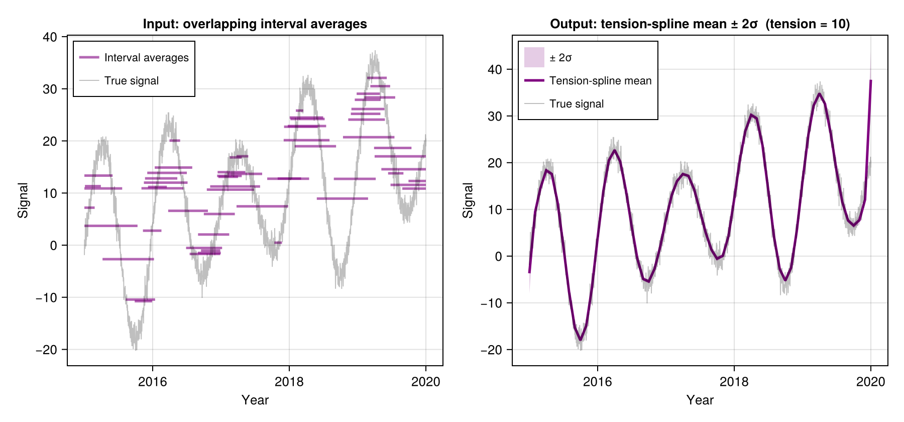

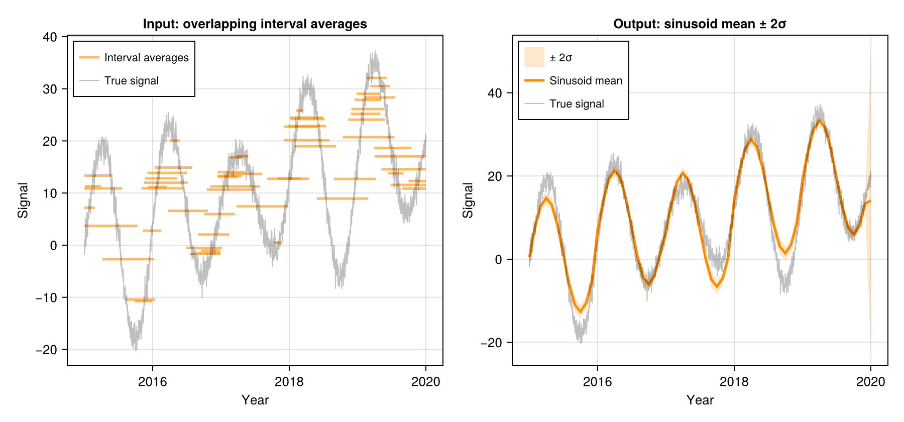
Sinusoid (Sinusoid)

Fits the parametric model:

x(t) = μ + β·(t − t̄) + γ(year) + A·sin(2πt) + B·cos(2πt)

where μ is the mean, β is a linear trend, γ(year) is a per-year anomaly, and A, B are annual seasonal amplitudes. All integrals are solved analytically — making this the fastest method.

result = disaggregate(Sinusoid(
    smoothness_interannual = 1e-2,   # ridge penalty on year-to-year anomalies
), y, t1, t2)

# Fitted parameters
using DimensionalData: metadata
md = metadata(result)
md[:amplitude]    # seasonal amplitude √(A²+B²)
md[:phase]        # peak time within year (fraction)
md[:trend]        # linear trend (units/year)
md[:interannual]  # Dict{Int,Float64} of per-year anomalies

Uncertainty: Spatially-varying sandwich std — lower where observations are dense, higher where they are sparse.

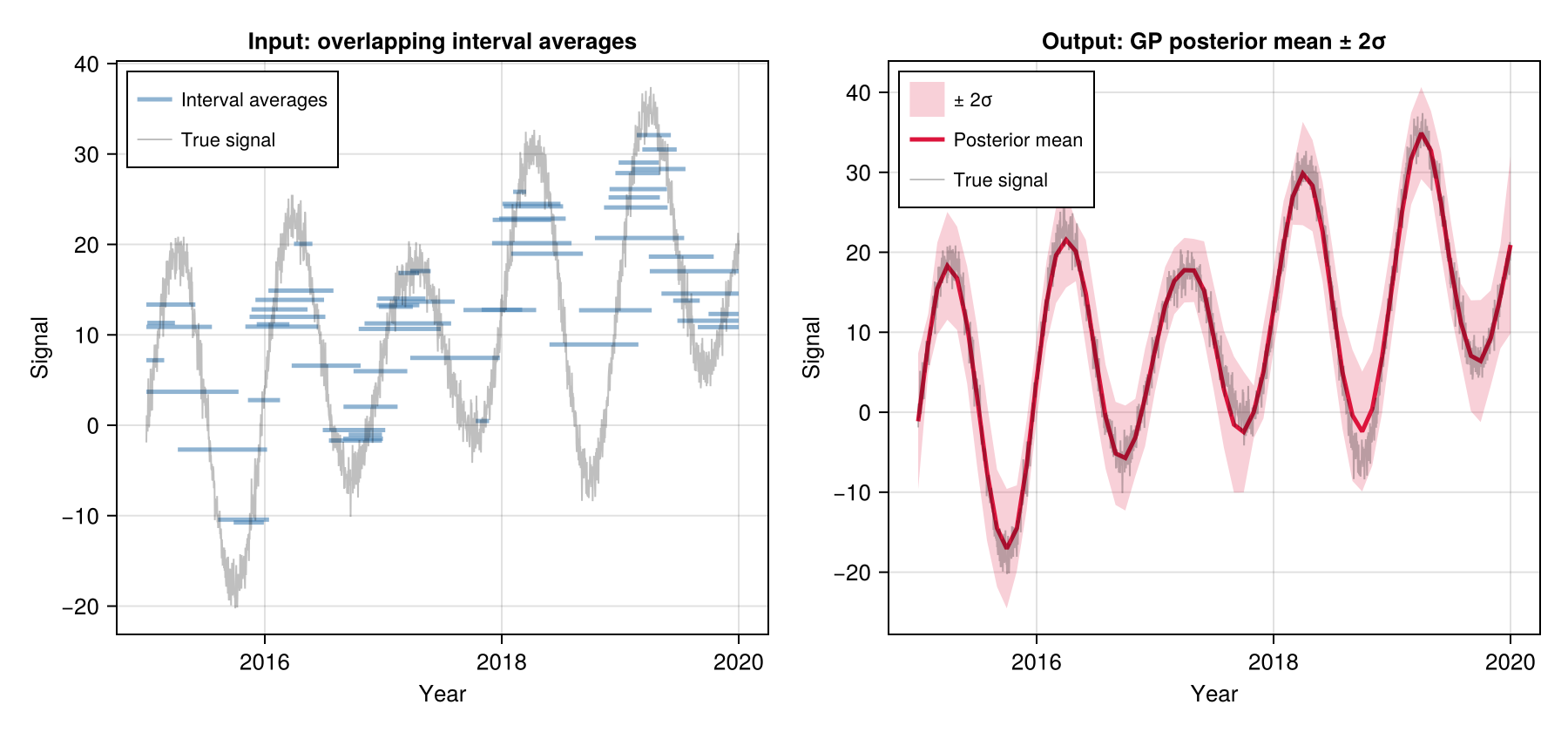
Gaussian Process (GP)

Models the signal as a Gaussian Process — a flexible probabilistic model encoding correlations through time. A sparse approximation keeps computation fast even for long records. Specify the correlation structure via a KernelFunctions.jl kernel.

using KernelFunctions

k = 15.0^2 * PeriodicKernel(r=[0.5]) * with_lengthscale(Matern52Kernel(), 3.0) +
     5.0^2 * with_lengthscale(Matern52Kernel(), 2.0)

result = disaggregate(GP(
    kernel           = k,
    obs_noise        = 4.0,   # initial noise variance σ² (auto-calibrated by default)
    n_quad           = 5,     # Gauss-Legendre quadrature points per interval
    calibrate_noise  = true,  # iteratively adjust obs_noise to match residual RMS
), y, t1, t2)

obs_noise calibration: When calibrate_noise=true (default), the method iteratively adjusts obs_noise to the value where the weighted RMS of interval-average residuals equals sqrt(obs_noise). This is an empirical Bayes fixed-point that makes the posterior mean insensitive to the initial obs_noise value — useful when obs_noise is hard to set a priori (e.g. when data units or scale are unknown). Set calibrate_noise=false to use obs_noise exactly as specified.

Uncertainty: Spatially-varying sandwich std — lower where observations are dense, higher where they are sparse.

Uncertainty

All three methods return the same type of std — a spatially-varying sandwich standard deviation:

std(t*) = σ̂ · sqrt(q(t*))

where σ̂ is the weighted residual RMS of predicted vs. observed interval averages (sqrt(Σ wᵢ rᵢ² / Σ wᵢ), with rᵢ = yᵢ − ŷᵢ) and q(t*) is a dimensionless coverage factor derived from the method's hat vector at time t*:

• Dense observation coverage → q(t*) < 1 → std(t*) < σ̂

• Sparse observation coverage → q(t*) > 1 → std(t*) > σ̂

This makes std comparable across methods and automatically reflects the temporal distribution of the input observations. When using loss_norm = :L1, both σ̂ and q(t*) are computed from the final IRLS solution.